Less data, more answers: AI inverse design for pixelated EM structures

This page summarises a paper I submitted to ASP-DAC 2027 (currently under anonymous review). Figures and numbers come from the manuscript.

In one sentence

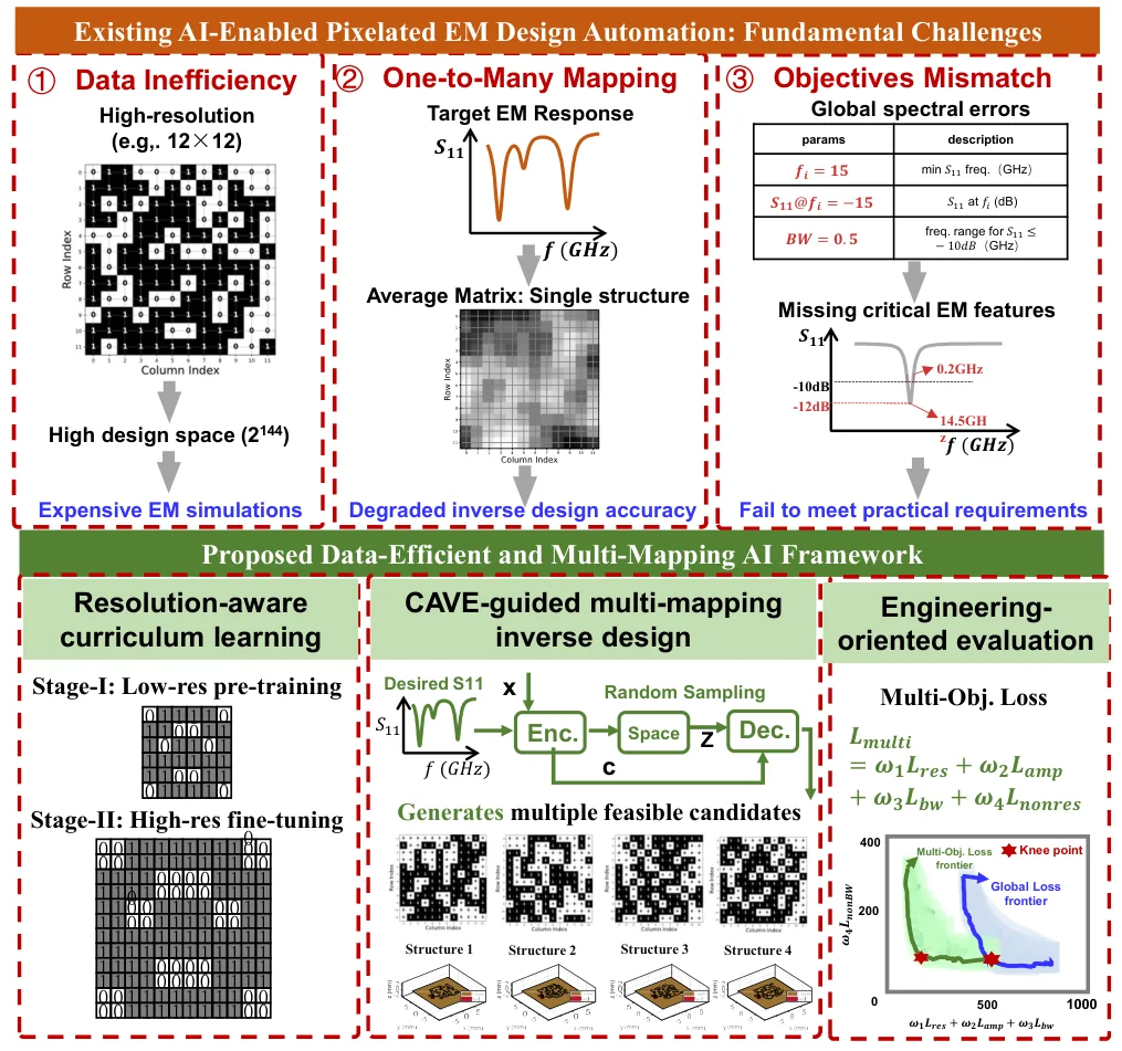
Give the model a target reflection response, and it draws a pixelated antenna patch directly — no manual parameter tuning, and no full-wave simulation at every step.

The patch is discretised into a 12×12 binary grid. Apart from the two feed pixels, every pixel can be copper or air. Higher resolution means more freedom, but also far more samples to simulate. This work addresses the three bottlenecks in between.

Three bottlenecks

① Data is expensive. A 12×12 grid has 142 free pixels — roughly 2^142 combinations. Enough high-resolution samples means thousands of full-wave simulations.

② One-to-many. One target response usually corresponds to many different structures. A deterministic network tends to output their “average”, which satisfies neither the specification nor the physics.

③ Misaligned objective. The usual loss is the error over the whole curve, while engineers care about whether the resonance lands at 18 GHz, how deep it is, whether the bandwidth is wide enough, and whether spurious resonances appear out of band. Two curves can look similar overall and still be unusable.

Method 1: resolution-aware curriculum learning (RACL)

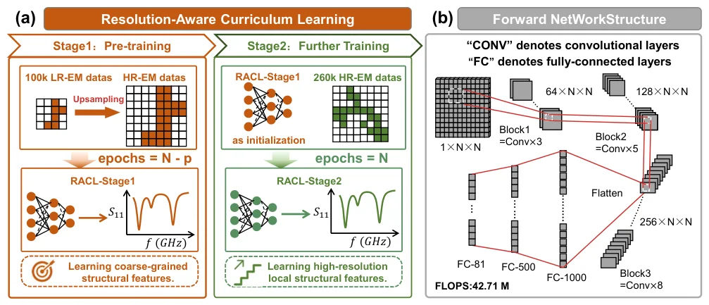
The idea resembles learning to write: get the shape roughly right on a small grid first, then refine it on a larger one.

The model is pre-trained on 6×6 low-resolution data to learn which shapes produce which responses; the low-resolution input is then nearest-neighbour upsampled to the high-resolution size, and the model is fine-tuned on high-resolution data. Every pixel stays binary throughout.

With the same 40k test set and comparable accuracy:

• data generation cost down 22.84% (416 h → 321 h)
• training cost down 11.52% (4054 s → 3587 s)
• forward-model accuracy essentially unchanged (R² 87.08% → 87.15%)

Method 2: Improved-CVAE, from one answer to many

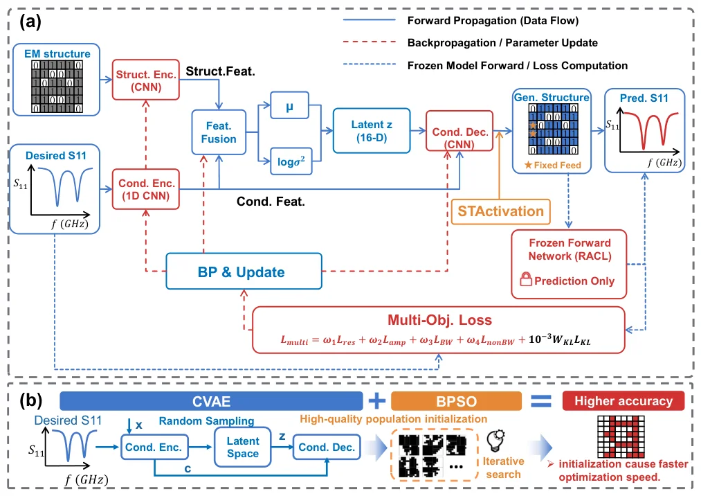
To handle one-to-many, deterministic prediction is replaced by conditional generation: a condition encoder reads the target S11, a structure encoder reads the real structure, both are fused into a 16-D latent z, and a conditional decoder maps z back to a structure.

Two details matter:

• ST activation: compresses the decoder’s continuous output towards 0/1, so the network emits a manufacturable pixel matrix rather than a greyscale image.
• KL warm-up: the KL term is ramped up over the first 15 epochs, so the model first learns the response-to-structure mapping and only then regularises the latent space. Generation diversity is more stable as a result.

The candidates are then used as the initial population for binary particle swarm optimisation (BPSO) — global generation followed by local search.

In this setting, design loss drops by 77.1% and 71.55% versus ANN and CNN baselines; compared with plain GA / BPSO search, optimisation time falls by 27.61% / 19.79% and design loss by 49.12% / 31.18%.

Method 3: engineering metrics inside the loss

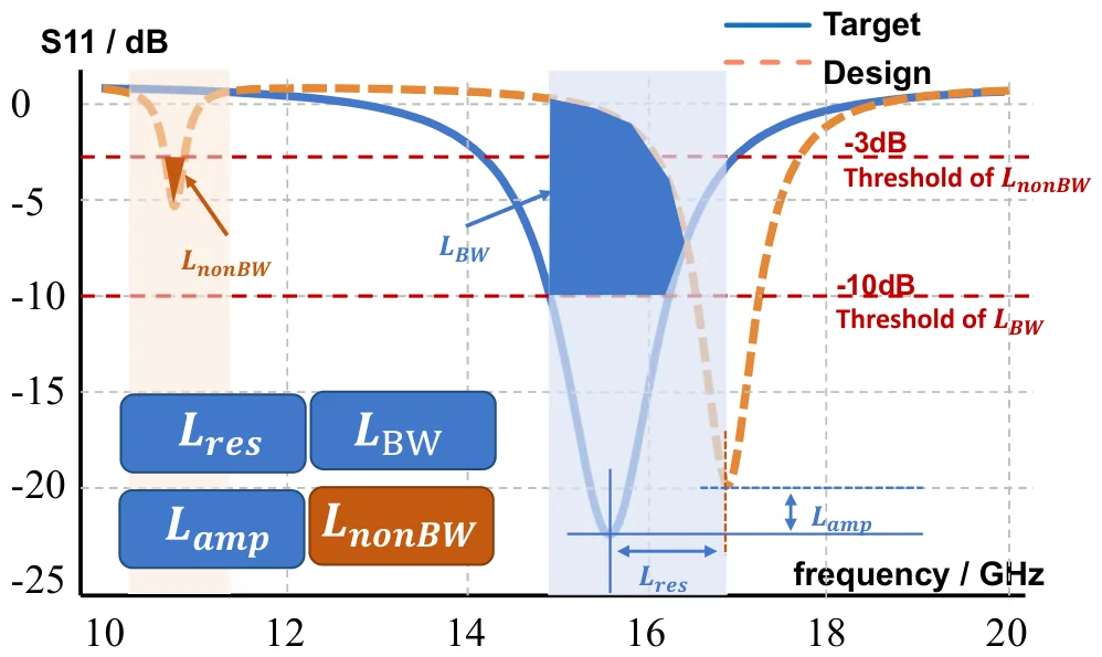
The total loss is split into four terms, each tied to something an engineer actually checks:

L = 30 · L_res + 1 · L_amp + 10 · L_BW + 8 · L_nonBW

• L_res: resonance-frequency deviation, located with a differentiable softmin instead of explicit peak picking.
• L_amp: resonance depth (S11 must be low enough).
• L_BW: matching must hold inside the target band.
• L_nonBW: no extra deep resonances out of band.

The optimisation target moves from “the whole curve looks alike” to “usable in engineering terms”.

Results

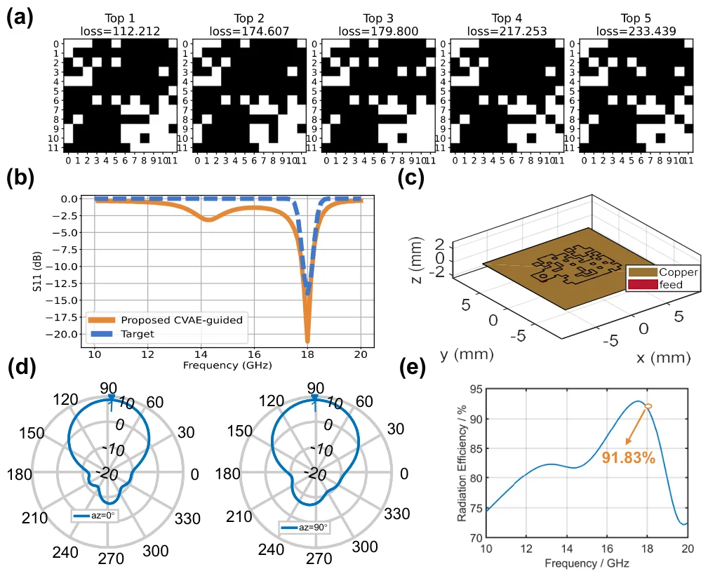
The single-band example targets 18 GHz: the final structure resonates at 18 GHz with S11 of −21.12 dB (target −14 dB), 0.5 GHz bandwidth (target 0.4 GHz) and peak radiation efficiency of 91.83%.

The dual-band example targets 13.5 GHz and 16.2 GHz: both resonances land near their targets with 0.375 GHz bandwidth, and radiation efficiency reaches 84.43% and 88.80% at the two frequencies.

One direction worth pursuing

Every term in the current loss is about the electromagnetic response — frequency, amplitude, bandwidth, out-of-band rejection. All of them live on the curve. None of them constrains the continuity of the structure itself.

So the model can return a patch that is electrically compliant but geometrically shattered: isolated pixels, disconnected copper islands, shapes that need extra post-processing before fabrication. Such solutions are legal in simulation, not in the fab.

Two possible fixes:

1. Write structural continuity as a differentiable regulariser and optimise it together with the EM loss — for example count neighbouring-pixel flips or connected copper components, so that “being one piece” becomes part of the objective rather than a post-filter.
2. Change how the structure is modelled. A pixel matrix is, in essence, a sequence, and Transformers handle long-range dependencies better than convolutions. They might capture global constraints such as “the current path has to stay connected” instead of only looking at local neighbourhoods.

Both are still at the idea stage — and they are roughly what I would like to work on next.

Next steps

• Find a continuity metric that is both cheap to compute and differentiable.
• Try sequence models (Transformer / state-space) in place of the CNN encoder.
• Close the loop between AI-generated candidates and EM co-optimisation, and measure how much simulation it actually saves.